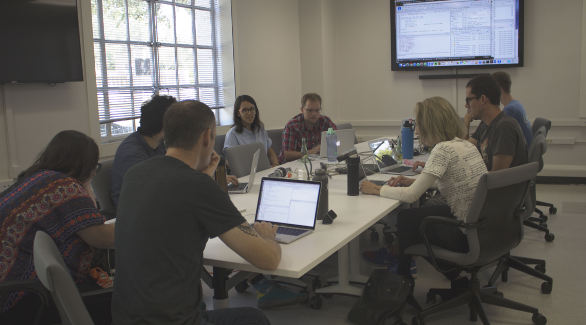
In the first workshop of the fall semester, Lars Hinrichs brought his knowledge of English Language and Linguistics to the DWRL for an introduction to R and Twitter.
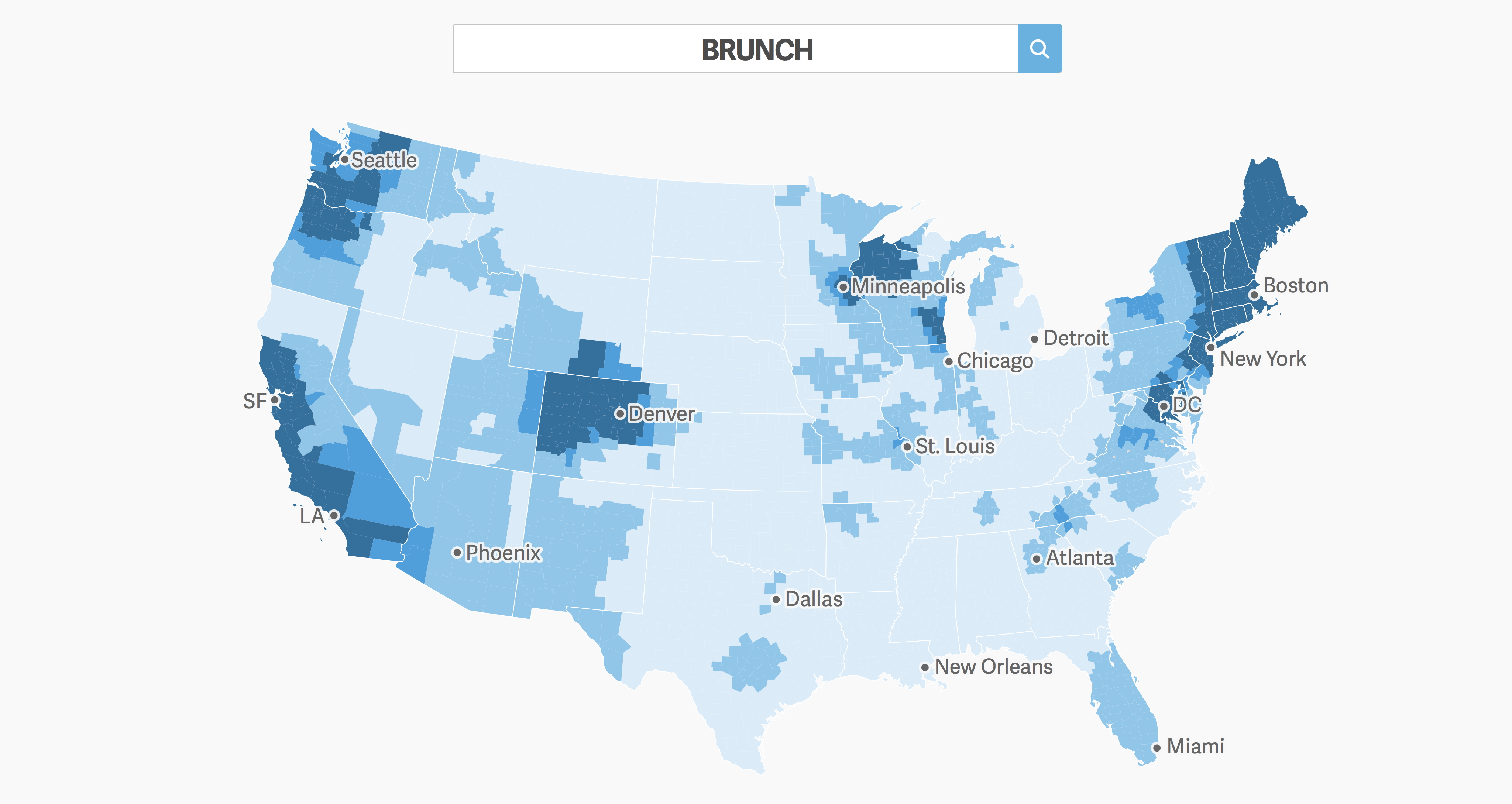
While Twitter’s reputation certainly preceded itself, the workshop began with an introduction to R — a necessary introduction for those of us unfamiliar with current research practices in the digital humanities. As a programming language, R is an open-source tool for statistical analysis and visualization. For a range of scholars interested in analyzing everything from traditional literature to live tweets, R has the ability to process text-based data and produce a variety of compelling visual analyses. To lead with an example, Lars cited a 2014 study that harvested billions of tweets in order to produce an interactive dialect map. Such an application of programming language allows us to understand what people are saying — and where.
Before we could accomplish anything so ambitious, we had to learn the humble basics of R. Specifically, we had to get a handle on communicating with R’s programming language and environment. Programming language centers around a series of typed inputs by the user that correlate with a series of outputs by the computer application. We experienced the process of assembling a dictionary of terms that allowed us to accomplish a small number of statistical tasks within R (i.e. storing values, creating data tables, running scripts). Ultimately, these simple skills were pertinent to our ultimate goal: collecting and statistically visualizing live tweets.
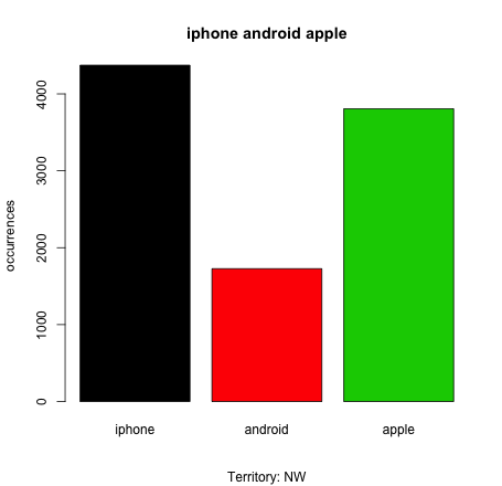
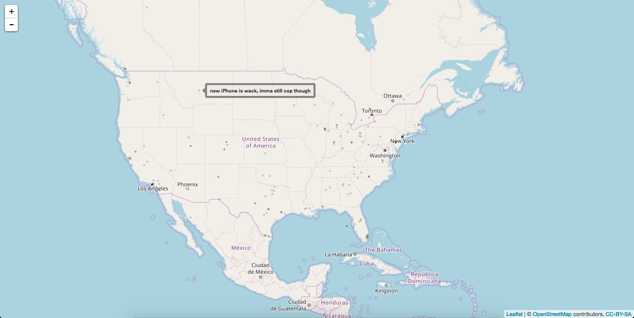
While we didn’t have the time to collect billions of tweets like the 2014 dialect study, we were able to link R with Twitter bots and — over the span of 45 minutes — collect a sample of about 12,000 tweets. For our exercise, we restricted our collection of live tweets based on two main parameters: keywords and locations. First, we only collected tweets containing at least one of the following keywords: “apple,” “iphone,” “android,” or “samsung.” Second, we only collected tweets posted within a certain GPS location — with each group of workshoppers focusing on a specific region of the continental United States.
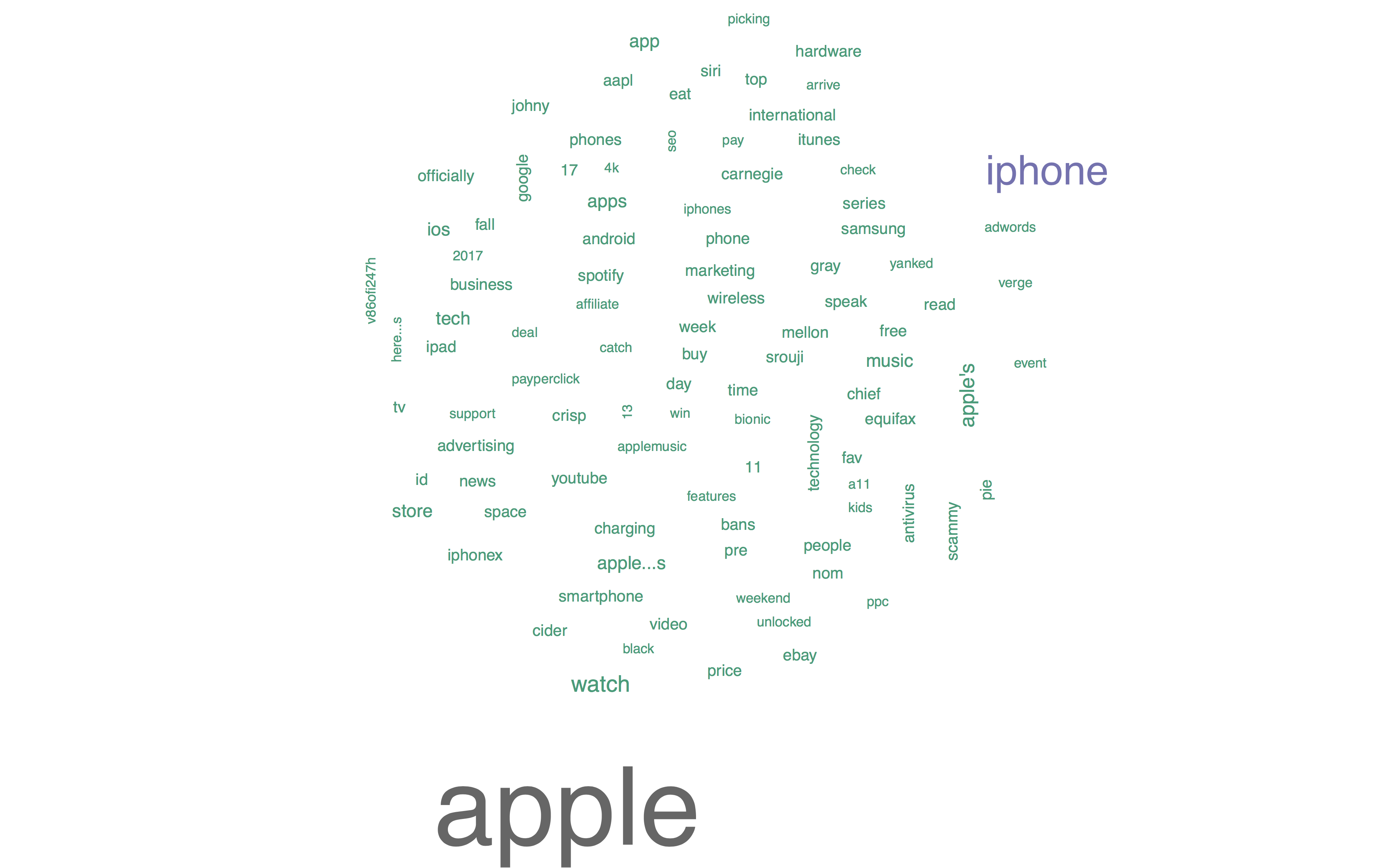
Having mined these tweets, we were then able to run a few basic visual analyses through R. You can check out a few examples of these below, but be sure to check out the word cloud for our keyword “apple,” in particular. This chart visualizes the words most frequently used in tweets containing the word “apple,” thus shedding light on a battle for attention: capital ‘A’ Apple vs. lowercase ‘a’ apple. Spoiler alert: the approach of Fall fever was no match for Apple’s recent iPhone announcement. Capital ‘A’ Apple dominated the word cloud, but lowercase ‘a’ apple squeezed in some little victories with ‘picking’, ‘cider’, and ‘nom’.